SmartSwitches are an exciting technology based on assumptions similar to SmartNICs. There is not much documentation on them, so Mario Baldi and I wrote a white paper that we distributed for the first time to the SmartNIC Summit in San Jose in April 2022.
Here is an excerpt on the history of network switching.
Enjoy
– Silvano
A History of Network Switches
1990s: Layer 2 Switches
Network switches (switches for short) are the evolution of network bridges whose behavior was defined by the Institute of Electrical and Electronics Engineers (IEEE) in the standard IEEE 802.1 to connect two or more Ethernet segments. Switch and switching are terms that do not exist in standards; they were introduced to indicate a multiport bridge.
Initially, switches were pure layer 2 devices that forwarded Ethernet frames without knowing their content and without modifying the frames, thus providing connectivity for the many layer 3 protocols deployed in those days. The forwarding model of layer 2 switches is straightforward and based on the exact lookup of the destination MAC address in a forwarding (or filtering) table; this is usually accomplished with a hashing table, which is easy to implement in hardware. Layer 2 switches do not require any configuration; the forwarding table is initially empty and is populated by associating the source MAC address of a frame being received with the port through which it is received - a technique called backward learning. When the lookup of the destination MAC address fails (i.e., the association of the MAC address with a port has not yet been done), the frame is forwarded on all ports other than the one it was received from - a technique named selective broadcast.
This forwarding technique works only on a tree topology because backward learning does not operate properly when frames travel along a loop and selective broadcast creates copies of frames traveling along a loop until the capacity of links and/or switches is saturated. On a mesh topology, the Spanning Tree protocol is deployed to block a set of ports that are not used to ensure that forwarding takes place on a tree. Blocking ports is inefficient from a bandwidth perspective because the corresponding links, although potentially capable of carrying traffic, are not being used. In the nineties, there was a lot of innovation around the spanning tree protocol trying to increase the overall network bandwidth, but all proposed solutions introduce significant complexity in the network design and configuration to ensure high bandwidth utilization.
2000s: The Introduction of Layer 3 Switches
In the 2000s, it became apparent that the only surviving layer 3 protocol was IPv4 (Internet Protocol version 4). Therefore, it made sense to bypass the limits of the Spanning Tree Protocol by implementing IPv4 routing into the switches. Layer 3 switches were born. IP forwarding does not require blocking any port in the network, hence it can take advantage of all the links in a network. Traditionally a Layer 3 switch forwards all traffic to a destination on the same path. However, a feature called ECMP (Equal Cost Multi Path) even enables to load balance traffic to each destination among multiple paths that are considered to have the same cost according to the routing protocol in use, like for example BGP (Border Gateway Protocol).
Appreciating the difference between layer 2 (L2) forwarding and layer 3 (L3) forwarding is essential to understanding why Layer 3 switches are substantially more complex than Layer 2 switches. At the IP level, forwarding is done packet-by-packet by looking up the destination IP address into a forwarding table with a technique called LPM (Longest Prefix Match), which is much more complex to implement in hardware than the exact, possibly hash-based, matching required in L2 switching. Deploying LPM enables the routing table not to include all the possible IP addresses, but just prefixes, thus allowing for larger networks without proportionally larger forwarding tables. A prefix is expressed as a combination of an IP address and a netmask to identify which bits in the address represent the prefix. Being 32 bit long, a netmask is cumbersome to write and not intuitive to understand; hence often the length of the prefix - or number of most significant bits in the address that represent the prefix - is explicitly indicated (e.g., /16, /24).
An entry of the forwarding table can be used to determine the forwarding information (e.g., the next hop and/or output interface) for any packet with a destination address that has that prefix in its most significant bits. If multiple entries match, the switch selects the one with the longest prefix: since it refers to a smaller set of addresses, it is somewhat more specific to the destination at hand.
This kind of forwarding is stateless since each packet is forwarded independently of previous packets. With the growing size of ICs (Integrated Circuits), more features were added to layer 3 switches, such as ACLs (Access Control Lists) to classify and filter packets, still in a stateless fashion, with limited scalability.
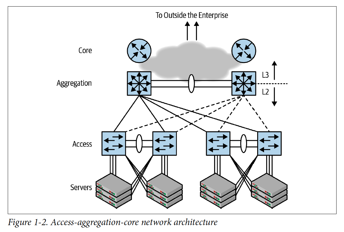
In terms of network design, the preferred topology was a Core-Aggregation-Access Design (picture courtesy of Dinesh Dutt): a mixture of layer 2 at the periphery and layer 3 in the network’s core, to allow layer 3 subnets to span across multiple edge switches. This allows, for example, Virtual Machine mobility among the servers connected to the same access switches. This design provided more aggregate bandwidth than a pure layer 2 approach, but still had a bottleneck in the two core and aggregation switches: traffic to all destinations not attached to the same pair of access switches must travel through the access switch identified as the root of the spanning tree.
2010: Modern L3 Switches
In the next decade, with the advent of even denser integrated circuits, layer 3 switches gained other functionality that can be grouped in three categories.
Clos Network and ECMP Support
Clos networks remove the bottleneck present in the core of the Core-Aggregation-Access Design. A Clos network is a multistage network that Charles Clos first formalized in 1952. It is a two-stage network in its simplest embodiment, like the one shown in the figure, but it can scale to an arbitrary number of stages.
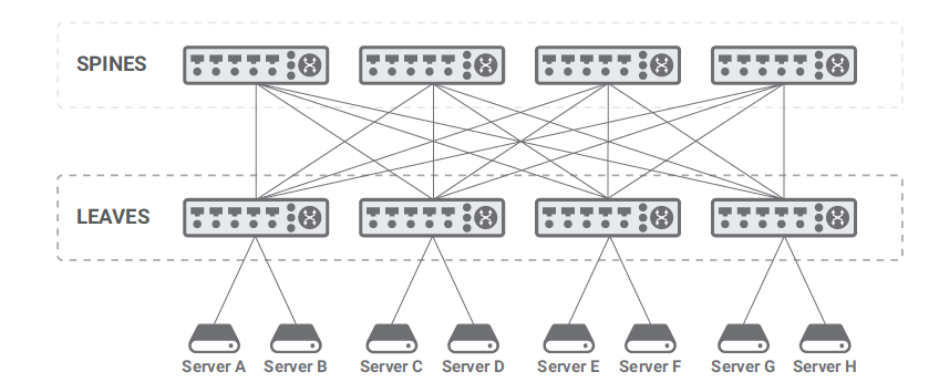
In their current usage and terminology, two-stage Clos networks have leaves (equivalent to access switches) and spines (equivalent to aggregation switches). The spines interconnect the leaves, and the leaves connect the network users. The network users are mostly, but not only the servers and can include network appliances, wide-area routers, gateways, and so on. No network users are attached to the spines.
The Clos topology is widely accepted in data center and cloud networks because it scales horizontally: adding more leaves allows to connect as many network users as needed, while adding more spines enables supporting larger amounts of East-West traffic. In fact, traffic to destinations not attached to the same leaf can transit through any of the spines (and corresponding link connecting the selected spine to the source and destination leaf). In order to enable this, both leaves and spines must be layer 3 switches (as layer 2 switches would block all leaf-spine links but one) and ensure that all spines are being used when forwarding packets. This is achieved through a technique called equal-cost multipath (ECMP) that stores multiple next hops (e.g., spines) for the same destination and load-balances forwarded packets to all of them.
Network Virtualization Support
Network virtualization enables the definition of multiple independent and separate virtual networks on a single physical network. In other words, although there is a single set of switches and links (physical network), multiple networks can be defined: the configuration (e.g., addressing scheme) of each network is independent from the others and the traffic is completely separated from the others.
Overlay networks are a common way to satisfy this requirement. An overlay network is a virtual network built on an underlay network, i.e., a physical infrastructure.
The underlay network’s primary responsibility is forwarding the overlay encapsulated packets (for example, using VXLAN encapsulation) across the underlay network efficiently using ECMP when available. The underlay provides a service to the overlay. In modern network designs, the underlay network is always an IP network (either IPv4 or IPv6) because we are interested in running over a Clos fabric that requires IP routing.
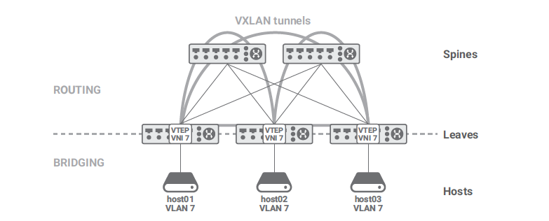
In overlays, it is possible to decouple the IP addresses used by the applications (overlay) from the IP addresses used by the infrastructure (underlay). The VMs that run a user application may use a few addresses from a customer IP subnet (overlay), whereas the servers that host the VMs use IP addresses that belong to the cloud provider infrastructure (underlay). VXLAN is probably the best-known encapsulation protocol for overlay networks.The points where packets are encapsulated/decapsulated are called VTEPs (VXLAN tunnel endpoints).
As we mentioned in the introduction, Core-Aggregation-Edge networks allowed layer 2 domains (that is, layer 2 broadcast domains) to span multiple switches. The VID (VLAN identifier) was the standard way to segregate the traffic from different users and applications. Each VLAN carried one or more IP subnets that were spanning multiple switches.
Clos network changed this by mandating routing between the leaves and the spines and limiting the layer 2 domains to the southern part of the leaves toward the hosts. The same is true for the IP subnets where the hosts are connected. VXLAN solves the problem of using Clos networks while at the same time propagating a layer 2 domain over them. In a nutshell, VXLAN carries a VLAN across a routed network. In essence, VXLAN enables seamless connectivity of servers by allowing them to continue to share the same layer 2 broadcast domain.
SDN Support
At the end of the previous century, all the crucial problems in networking were solved. On my bookshelf, I still have a copy of Interconnections: Bridges and Routers by Radia Perlman dated 1993. In her book, Perlman presents the spanning tree protocol for bridged networks, distance vector routing, and link-state routing: all the essential tools that we use today to build a network. During the following two decades, there have been improvements, but they were minor, incremental. The most significant change has been the dramatic increase in link speed.
In 2008, Professor Nick McKeown and others published their milestone paper on OpenFlow. Everybody got excited and thought that with software-defined networking (SDN), networks would change forever. They did, but it was a transient change; many people tried OpenFlow, but few adopted it. Five years later, most of the bridges and routers were still working as described by Perlman in her book.
But two revolutions had started:
- A distributed control plane with open API
- A programmable data plane
The second one was not successful because it was too simple and didn’t map well to hardware. However, it created the condition for the development of P4 architecture to address those issues. OpenFlow impacted even more host networking, where the SDN concept is used in a plethora of solutions.
SDN enables virtualized networks with a less complex overlay not based on running control protocols like BGP, but programmed through an SDN controller.
Scalability Considerations
These switches have impressive performance in terms of bandwidth and PPS (Packet Per Second) but they are substantially stateless devices that are not idoneous to implement stateful services like firewall, NAT, load balancing, etc. They also have scalability issues in the number of routes and ACLs that they can support.
Scalability is critical because each virtual network has its addressing space that cannot be aggregated with one of the others and its own separate tables for services like ACL, NAT, etc.. Hence, even though the virtual topology of virtualized networks may be simpler than the physical topology, and hence routing tables smaller than the ones of the physical network, still the amount of memory required for routing tables and data structures for other services increases the size of routing tables. Moreover, VTEP mapping requires large tables that are not present in traditional switches that do not support network virtualization.
2020: SmartSwitches (Distributed Service Switches)
SmartSwitches, a.k.a Distributed Service Switches, add to the state of the art layer 3 switches a rich collection of wire-rate stateful services, e.g., firewall, LB (Load Balancer), NAT (Network Address Translation, TAP (Test Access Point) Network (traffic observability), streaming telemetry, etc. A SmartSwitch can apply these services both to the underlay network and to the overlay network. In the second case, they are typically colocated with the VTEPs.
To effectively support these services, SmartSwitches have a different forwarding mechanism that is stateful: decision of what to do with the packet may depend on previous packets of the same communication. Hence, each packet between host A and host B is processed as a part of a session between A and B that comprises two unidirectional flows: one from A to B and one from B to A. The term session applies as well to connection oriented protocols like TCP or connectionless protocols like UDP.
The concept of session is important because in many cases reaching the forwarding decision (whether to forward the packet and if so how) requires complex processing of one or more packets and then remains the same for subsequent packets of the same communication.
The stateful forwarding mechanism is also called cache-based forwarding. It relies on a flow cache, a binary data structure capable of “exact” matching packets belonging to a particular flow. The word “exact” implies a binary match easier to implement both in hardware or software, unlike a ternary match, such as LPM. The flow cache contains an entry for each flow, i.e., two entries per session. The flow can be defined with an arbitrary number of fields, thus supporting IPv4 and IPv6 addresses, different encapsulations, policy routing, and firewalling.
Cache entry contains information needed to forward the packet (e.g., layer 2 and/or layer 3 address of the next hop, type of encapsulation, etc.).
The separate initial processing that leads to the forwarding decision may create new cache entries. When a packet is received by the switch, if it does not match any entry in the flow cache (a “miss”) it is processed according to the initial processing. Otherwise (“hit”), it is forwarded according to the information in the matching flow cache entry.
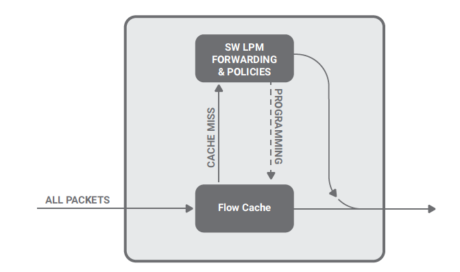
The above figure shows the organization of this solution. Any packet that causes a miss in the flow cache is redirected to a software process that applies a complete decision process and forwards or drops the packet accordingly. This software process also adds two entries in the flow cache (dashed line) for the session, so that subsequent packets can be forwarded or dropped as the previous packets of the same flow.
Because the processing of initial packets (misses) is so clearly separated from the processing of the following packets (hits), it can be implemented independently and possibly on a separated execution engine. For example, hits could be processed by a specialized integrated circuit or an application specific processor (hardware data path), while misses could be processed by software running on a general purpose CPU (software data path).
Let’s suppose that an average flow is composed of 500 packets: one will hit the software process, and the remaining 499 will be processed directly in hardware with a speed-up factor of 500 compared to a pure software solution. In other words, cache-based forwarding allows one to take advantage of the flexibility of software with the performance of hardware. Of course, this solution should guarantee that packets processed in software and hardware do not get reordered.
Since in cache-based forwarding the handling of the first packet of a flow or session can be implemented completely independently from the handling of subsequent packets, when evaluating the performance of a SmartSwitch we look at two different indexes:
- Connections Per Second (CPS) offers an indication of the performance in processing the initial packet of each flow.
- Packet Per Second (PPS) provides a measure of the performance in processing other packets.
In specific use cases, complex and time consuming processing is allowed on the first packet to decide whether and how a flow should be forwarded without affecting the throughput in terms of PPS.
Scalability Considerations
This architecture requires that the SmartSwitches have a large volume of high-speed memory to store all the flow descriptors, the ACLs, and the routes. Cloud providers have a large number of tenants each with their virtual network. Even if routing and access control lists (ACLs) requirements for each tenant are moderate, when multiplied by the number of tenants, there is an explosion in the number of routes and ACLs, which can be difficult to accommodate on the host with traditional table lookups. It is not unreasonable to support millions of routes and ACLs and tens of millions of flows. If the flow descriptor is, let’s say, 256 bytes, and we have ten million, the flow cache consumes 2.5 GB of memory. When we add the size of the route table, the ACL table, intermediate data structure and code, it is not unreasonable to use 8 to 16 GB of memory. This size of memory cannot be integrated on-chip, and therefore external memory needs to be used. Multiple DDR busses are required to obtain high performance, with DDR5 at the highest possible frequency being desirable. It helps that, with the exception of the flow table, the rest of information/tables is needed only for processing misses, which is a small fraction of the overall traffic.